Spatial correlation modeling of environmental extremes with HazardMaps

Overview

HazardMaps provides a unified workflow for spatial dependence modeling of environmental extremes — from raw gridded datasets to spatially coherent pseudoscenarios. The package supports regular longitude-latitude grids (e.g. ERA5, Copernicus) and rotated curvilinear grids (e.g. EURO-CORDEX) without any change in the user interface.

Example dataset. This vignette uses daily maximum wind-gust speed over Northeast Italy as a running example. The workflow applies unchanged to any gridded environmental variable: precipitation, temperature, wave height, etc. The package was developed as part of the research presented in Clavijo Mesa et al. (2026a, 2026b), whose datasets are included as built-in example files. Users who need to prepare raw Copernicus or EURO-CORDEX downloads before using the package can find helper R scripts in inst/scripts/, accessible via system.file("scripts", package = "HazardMaps").

Two datasets are used throughout:

Copernicus — regular longitude-latitude grid, ERA5-based, 195 cells, 1994–2021
EURO-CORDEX — rotated curvilinear grid, RCM simulation, 1872 cells (1568 land), 1970–2005

The workflow has seven steps:

Ingest and prepare data
Select extreme-event days
Fit marginal distributions
Estimate spatial dependence
Fit copula and stochastic field models
Simulate pseudoscenarios
Validate with cluster-size statistics

library(HazardMaps)

Step 1 — Ingest and prepare data

The starting point is a CF-convention NetCDF file. hm_read_netcdf() reads it and detects the grid type automatically — no configuration needed.

wind_cop <- hm_read_netcdf(
  system.file("extdata", "Copernicus_dailymax_1994_2021.nc",
              package = "HazardMaps"),
  var = "i10fg"
)

wind_euc <- hm_read_netcdf(
  system.file("extdata", "EuroCordex_wsgsmax_1970_2005.nc",
              package = "HazardMaps"),
  var = "wsgsmax"
)

wind_cop$meta$grid_type
#> [1] "regular"
wind_euc$meta$grid_type
#> [1] "rotated"

hm_standardize_coords() flattens the coordinate arrays into a single data.frame with one row per grid cell — the format all downstream functions expect. hm_decode_time() converts CF-style time values (e.g. “days since 1970-01-01”) to R Date objects.

wind_cop <- hm_standardize_coords(wind_cop)
wind_cop <- hm_decode_time(wind_cop)
wind_cop <- hm_get_grid_geometry(wind_cop)

wind_euc <- hm_standardize_coords(wind_euc)
wind_euc <- hm_decode_time(wind_euc)
wind_euc <- hm_get_grid_geometry(wind_euc)

cat("Copernicus: ", nrow(wind_cop$coords), "cells |",
    length(wind_cop$time), "days\n")
#> Copernicus:  195 cells | 10226 days
cat("EURO-CORDEX:", nrow(wind_euc$coords), "cells |",
    length(wind_euc$time), "days\n")
#> EURO-CORDEX: 1872 cells | 13149 days

hm_plot_spatial_domain() visualises the study area. It draws the correct cell geometry automatically — straight lines for regular grids, curvilinear lines for rotated grids.

hm_plot_spatial_domain(wind_cop, dataset = "copernicus",
                       title = "Copernicus domain", show_map = TRUE)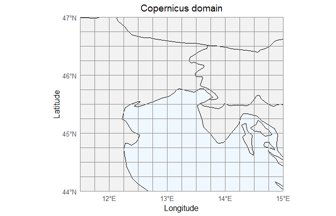

Copernicus regular grid domain.

hm_plot_spatial_domain(wind_euc, dataset = "eurocordex",
                       title = "EURO-CORDEX domain", show_map = TRUE)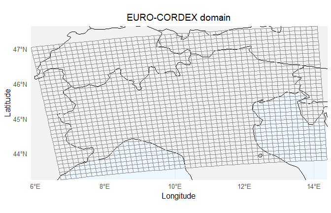

EURO-CORDEX rotated grid domain.

Step 2 — Select extreme-event days

Only days with at least one grid cell at or above a threshold are kept. Everything below the threshold is noise for dependence modeling purposes.

wind_cop_ext <- hm_select_extreme_events(wind_cop, threshold = 25)
wind_euc_ext <- hm_select_extreme_events(wind_euc, threshold = 25)

cat("Copernicus: ", wind_cop_ext$meta$filter$n_days_retained,
    "extreme-event days out of", wind_cop_ext$meta$filter$n_days_original, "\n")
#> Copernicus:  382 extreme-event days out of 10226
cat("EURO-CORDEX:", wind_euc_ext$meta$filter$n_days_retained,
    "extreme-event days out of", wind_euc_ext$meta$filter$n_days_original, "\n")
#> EURO-CORDEX: 5635 extreme-event days out of 13149

hm_plot_exceedance() maps how often each cell exceeded the threshold over the full period.

hm_plot_exceedance(wind_cop, threshold = 25, metric = "count",
                   dataset = "copernicus", show_map = TRUE,
                   title = "Wind-gust exceedance count — Copernicus")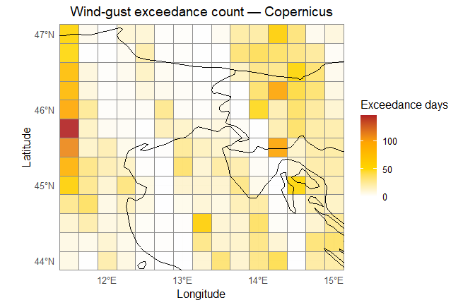

Exceedance count — Copernicus.

hm_plot_exceedance(wind_euc, threshold = 25, metric = "count",
                   dataset = "eurocordex", show_map = TRUE,
                   title = "Wind-gust exceedance count — EURO-CORDEX")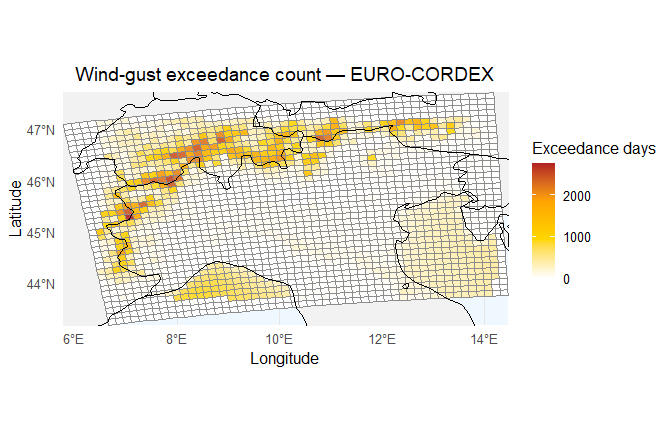

Exceedance count — EURO-CORDEX.

hm_plot_exceedance_time() shows whether the frequency of extreme events changes over the observation period.

hm_plot_exceedance_time(wind_cop, threshold = 25, by = "year",
                        title = "Extreme-event days per year — Copernicus")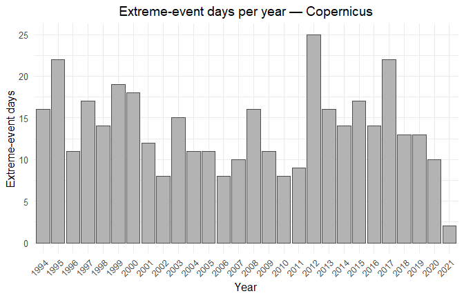

Extreme-event days per year — Copernicus.

hm_plot_exceedance_time(wind_euc, threshold = 25, by = "decade",
                        title = "Extreme-event days per decade — EURO-CORDEX")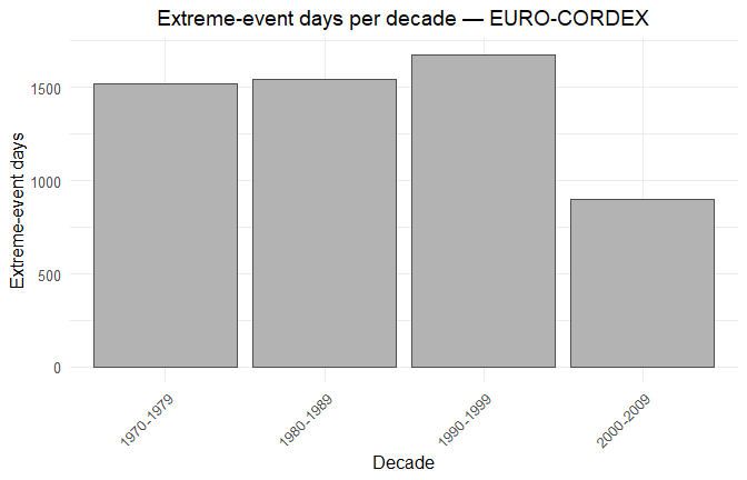

Extreme-event days per decade — EURO-CORDEX.

Step 3 — Fit marginal distributions

Before estimating spatial dependence, each cell needs its own marginal distribution. This separates the marginal behavior from the dependence structure — a standard approach in multivariate extreme-value analysis.

hm_to_matrix() reshapes the data into a time-by-cell matrix. hm_filter_land_cells() removes columns with no valid data — mandatory for EURO-CORDEX, whose domain includes sea cells.

obs_cop <- hm_to_matrix(wind_cop_ext)
obs_euc <- hm_to_matrix(wind_euc_ext)

obs_cop <- hm_filter_land_cells(obs_cop)
obs_euc <- hm_filter_land_cells(obs_euc)

cat("Copernicus matrix :", nrow(obs_cop), "days x", ncol(obs_cop), "cells\n")
#> Copernicus matrix : 382 days x 195 cells
cat("EURO-CORDEX matrix:", nrow(obs_euc), "days x", ncol(obs_euc), "cells\n")
#> EURO-CORDEX matrix: 5635 days x 1568 cells

hm_fit_marginals() fits six candidate families to each cell by maximum likelihood and selects the best by BIC. The six families are: Weibull, Gamma, Lognormal, Gumbel, Zero-truncated Gaussian, and Zero-truncated Laplace.

marginals_cop <- hm_fit_marginals(obs_cop, criterion = "bic")
marginals_euc <- hm_fit_marginals(obs_euc, criterion = "bic")

cat("Copernicus — best distribution per cell:\n")
#> Copernicus — best distribution per cell:
print(sort(table(marginals_cop$best_dist), decreasing = TRUE))
#> 
#> weibull   gamma   tnorm   lnorm  gumbel 
#>     124      44      17       9       1

cat("\nEURO-CORDEX — best distribution per cell:\n")
#> 
#> EURO-CORDEX — best distribution per cell:
print(sort(table(marginals_euc$best_dist), decreasing = TRUE))
#> 
#>  weibull    tnorm    gamma    lnorm tlaplace 
#>     1138      284      112       23       11

What to look for. Weibull dominates in both datasets — this is expected for wind-gust extremes. The spatial map below shows which cells deviate from Weibull and why: coastal cells and Alpine valleys tend to favour Gamma or Zero-truncated Gaussian due to their different tail behavior.

hm_plot_best_dist(wind_cop_ext, marginals_cop,
                  title = "Best-fitting marginal — Copernicus",
                  show_map = TRUE)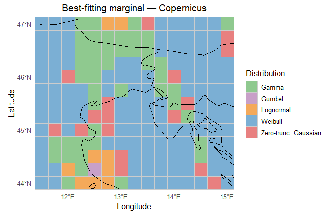

Best-fitting distribution at each cell — Copernicus.

wind_euc_land        <- wind_euc_ext
wind_euc_land$coords <- attr(obs_euc, "coords")

hm_plot_best_dist(wind_euc_land, marginals_euc,
                  title = "Best-fitting marginal — EURO-CORDEX",
                  show_map = TRUE)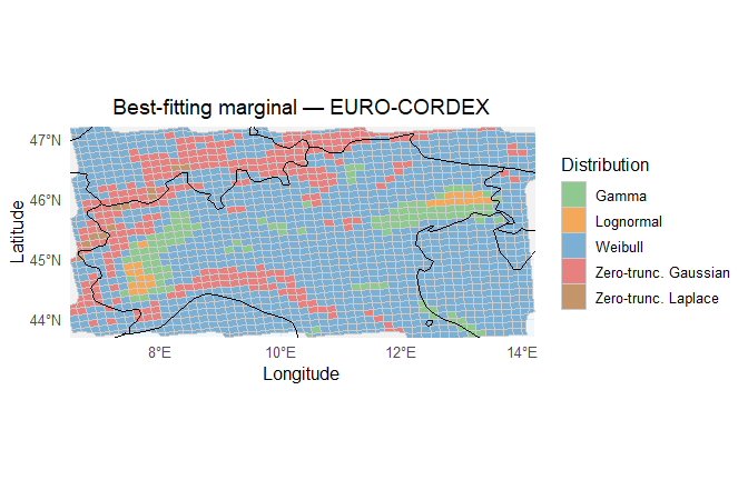

Best-fitting distribution at each cell — EURO-CORDEX.

hm_plot_dist_frequency(marginals_cop,
                       title = "Distribution frequency — Copernicus")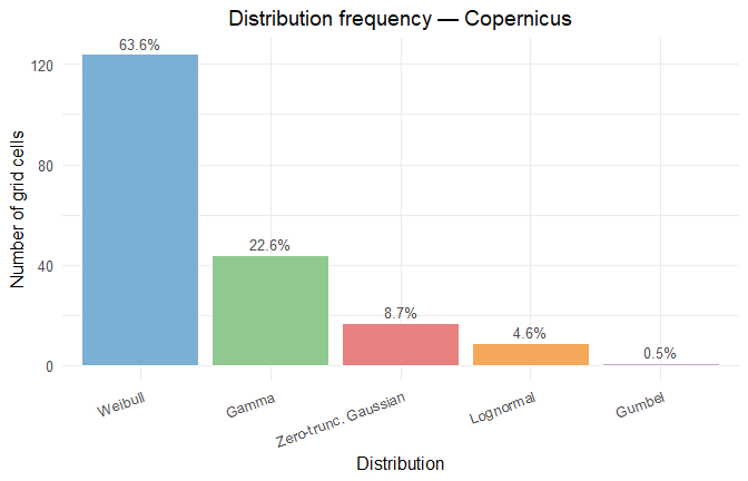

Frequency of best-fitting families across all cells.

hm_plot_dist_frequency(marginals_euc,
                       title = "Distribution frequency — EURO-CORDEX")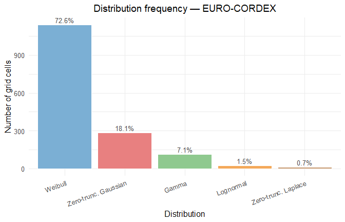

Frequency of best-fitting families across all cells.

The Probability Integral Transform (PIT) converts each observation to the uniform scale using its fitted CDF, then to Gaussian scores via the probit transform. The Gaussian scores (Z) feed the spatial dependence estimation; the uniform values (U) feed the copula.

pit_cop <- hm_pit_transform(obs_cop, marginals_cop)
pit_euc <- hm_pit_transform(obs_euc, marginals_euc)

cat("Copernicus — cells transformed:", pit_cop$n_cells_ok,
    "| skipped:", pit_cop$n_cells_skipped, "\n")
#> Copernicus — cells transformed: 195 | skipped: 0
cat("EURO-CORDEX — cells transformed:", pit_euc$n_cells_ok,
    "| skipped:", pit_euc$n_cells_skipped, "\n")
#> EURO-CORDEX — cells transformed: 1568 | skipped: 0

Step 4 — Estimate spatial dependence

The empirical spatial correlation is measured with Kendall’s τ, which is rank-based and does not assume any distribution for the data.

hm_distance_matrix() computes the great-circle distance in kilometres between every pair of cells. hm_empirical_kendall() estimates the pairwise Kendall correlation from the Gaussian scores.

Computational note. For large grids (> 500 cells), computing all N(N-1)/2 pairs is expensive. Use cell_idx to pass a representative subsample — as done here for EURO-CORDEX.

distances_cop <- hm_distance_matrix(attr(obs_cop, "coords"))
kendall_cop   <- hm_empirical_kendall(pit_cop$Z)

land_idx      <- which(!is.na(marginals_euc$best_dist))[1:50]
distances_euc <- hm_distance_matrix(attr(obs_euc, "coords")[land_idx, ])
kendall_euc   <- hm_empirical_kendall(pit_euc$Z, cell_idx = land_idx)

hm_empirical_correlogram() bins the pairwise correlations by distance to produce a smooth summary of how correlation decays with separation.

corg_cop <- hm_empirical_correlogram(kendall_cop, distances_cop, n_bins = 20)
corg_euc <- hm_empirical_correlogram(kendall_euc, distances_euc, n_bins = 15)

hm_plot_correlogram(corg_cop,
                    title = "Empirical correlogram — Copernicus")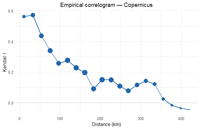

Empirical spatial correlogram for both datasets.

hm_plot_correlogram(corg_euc,
                    title = "Empirical correlogram — EURO-CORDEX (50-cell subsample)")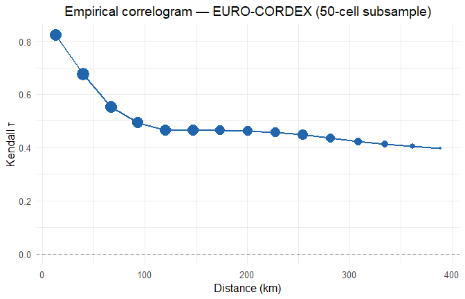

Empirical spatial correlogram for both datasets.

Interpretation. Correlation is highest at short distances (~0.75–0.80) and decreases steadily with increasing separation, reaching near-zero beyond 250–300 km. This pattern confirms strong local spatial dependence and weak long-range dependence — consistent with synoptic-scale windstorm events that affect areas of 50–200 km.

Step 5 — Fit dependence models

Two model families are available and compared.

Copula models

Vine copulas decompose the joint distribution of all cells into a cascade of bivariate copulas. Three structures are available: C-vine (one central node drives all others), D-vine (a chain structure), and Gaussian (elliptical baseline).

uniform_small   <- pit_cop$U[, 1:30]
marginals_small <- marginals_cop[1:30, ]

copula_cvine <- hm_fit_copula(uniform_small, type = "cvine")
copula_dvine <- hm_fit_copula(uniform_small, type = "dvine")
copula_gauss <- hm_fit_copula(uniform_small, type = "gaussian")

cat("Cells:", copula_cvine$n_cells,
    "| Observations:", copula_cvine$n_obs, "\n")
#> Cells: 30 | Observations: 382

Stochastic field model

The stochastic field approach fits a parametric covariance function directly to the empirical correlogram, then generates realisations via the Karhunen-Loève Expansion (KLE). Four covariance families are compared automatically: Matérn, Exponential, Gaussian, and Spherical.

sf_model_cop <- hm_fit_correlation_model(corg_cop)
sf_model_euc <- hm_fit_correlation_model(corg_euc)

cat("Copernicus  — best:", sf_model_cop$best_family,
    "| RMSE:", round(sf_model_cop$best_rmse, 4), "\n")
#> Copernicus  — best: matern | RMSE: 0.0541
cat("EURO-CORDEX — best:", sf_model_euc$best_family,
    "| RMSE:", round(sf_model_euc$best_rmse, 4), "\n")
#> EURO-CORDEX — best: exponential | RMSE: 0.0737

cat("\nFamily comparison — Copernicus:\n")
#> 
#> Family comparison — Copernicus:
print(sf_model_cop$all_fits)
#>        family     rmse converged
#> 1      matern 0.054148      TRUE
#> 2 exponential 0.056362      TRUE
#> 3    gaussian 0.069971      TRUE
#> 4   spherical 0.066445      TRUE

cat("\nFitted parameters:\n")
#> 
#> Fitted parameters:
print(round(sf_model_cop$best_params, 4))
#>      range smoothness     nugget 
#>   116.4797     0.1997     0.0000

How the best family is chosen. All four covariance families are fitted by weighted least squares to the empirical correlogram. The one with the lowest RMSE is selected automatically and stored in model$best_family. No manual choice is needed.

Step 6 — Simulate pseudoscenarios

Each model generates a matrix of synthetic extreme-event fields. Every row is one spatially coherent scenario — a plausible simultaneous wind-gust intensity at all grid cells.

scenarios_cvine <- hm_simulate_copula(copula_cvine, marginals_small,
                                       n_scenarios = 500L, seed = 42L)
scenarios_dvine <- hm_simulate_copula(copula_dvine, marginals_small,
                                       n_scenarios = 500L, seed = 42L)
scenarios_gauss <- hm_simulate_copula(copula_gauss, marginals_small,
                                       n_scenarios = 500L, seed = 42L)

cat("Copula scenarios — dimensions:", dim(scenarios_cvine)[1], "x",
    dim(scenarios_cvine)[2], "\n")
#> Copula scenarios — dimensions: 500 x 30
cat("Value range: [",
    round(min(scenarios_cvine, na.rm = TRUE), 2), ",",
    round(max(scenarios_cvine, na.rm = TRUE), 2), "] m/s\n")
#> Value range: [ 2.22 , 41.62 ] m/s

scenarios_sf <- hm_simulate_sf_kle(
  sf_model_cop, distances_cop, marginals_cop,
  n_scenarios = 500L, var_retain = 0.95, seed = 42L
)

cat("SF scenarios — dimensions:", dim(scenarios_sf)[1], "x",
    dim(scenarios_sf)[2], "\n")
#> SF scenarios — dimensions: 500 x 195
cat("KLE modes retained:", attr(scenarios_sf, "k_modes"),
    "| Variance explained:", round(attr(scenarios_sf, "var_explained"), 3), "\n")
#> KLE modes retained: 165 | Variance explained: 0.951
cat("Value range: [",
    round(min(scenarios_sf, na.rm = TRUE), 2), ",",
    round(max(scenarios_sf, na.rm = TRUE), 2), "] m/s\n")
#> Value range: [ 0.98 , 43.97 ] m/s

Step 7 — Validate with cluster-size statistics

A good dependence model should reproduce the spatial footprint of observed events — not just the marginal distribution of each cell in isolation.

hm_cluster_size() counts, for each day, how many cells simultaneously exceeded the threshold. This gives a simple but powerful summary of the spatial extent of each event.

cluster_obs <- hm_cluster_size(obs_cop, threshold = 25,
                                time = attr(obs_cop, "time"))

cat("Observed spatial footprint (Copernicus):\n")
#> Observed spatial footprint (Copernicus):
print(summary(cluster_obs$cluster_size))
#>    Min. 1st Qu.  Median    Mean 3rd Qu.    Max. 
#>   1.000   2.000   4.000   8.885  10.000 138.000

The same statistic applied to the simulated scenarios reveals how well each model reproduces the observed footprint distribution.

cluster_cvine <- hm_cluster_size(scenarios_cvine, threshold = 25)
cluster_dvine <- hm_cluster_size(scenarios_dvine, threshold = 25)
cluster_gauss <- hm_cluster_size(scenarios_gauss, threshold = 25)
cluster_sf    <- hm_cluster_size(scenarios_sf,    threshold = 25)

footprint_table <- data.frame(
  Model  = c("Observed", "C-vine", "D-vine", "Gaussian", "SF (Matérn)"),
  Mean   = round(c(mean(cluster_obs$cluster_size),
                   mean(cluster_cvine$cluster_size),
                   mean(cluster_dvine$cluster_size),
                   mean(cluster_gauss$cluster_size),
                   mean(cluster_sf$cluster_size)), 2),
  Median = round(c(median(cluster_obs$cluster_size),
                   median(cluster_cvine$cluster_size),
                   median(cluster_dvine$cluster_size),
                   median(cluster_gauss$cluster_size),
                   median(cluster_sf$cluster_size)), 2),
  Max    = c(max(cluster_obs$cluster_size),
             max(cluster_cvine$cluster_size),
             max(cluster_dvine$cluster_size),
             max(cluster_gauss$cluster_size),
             max(cluster_sf$cluster_size))
)

print(footprint_table, row.names = FALSE)
#>        Model Mean Median Max
#>     Observed 8.88      4 138
#>       C-vine 2.22      0  24
#>       D-vine 2.41      0  23
#>     Gaussian 2.49      0  27
#>  SF (Matérn) 8.39      6  66

all_clusters <- rbind(
  data.frame(model = "Observed",    size = cluster_obs$cluster_size),
  data.frame(model = "C-vine",      size = cluster_cvine$cluster_size),
  data.frame(model = "D-vine",      size = cluster_dvine$cluster_size),
  data.frame(model = "Gaussian",    size = cluster_gauss$cluster_size),
  data.frame(model = "SF (Matérn)", size = cluster_sf$cluster_size)
)

all_clusters$model <- factor(
  all_clusters$model,
  levels = c("Observed", "C-vine", "D-vine", "Gaussian", "SF (Matérn)")
)

ggplot2::ggplot(all_clusters,
                ggplot2::aes(x = size, colour = model)) +
  ggplot2::stat_ecdf(linewidth = 0.9) +
  ggplot2::scale_colour_manual(
    values = c("Observed"    = "black",
               "C-vine"      = "#2166AC",
               "D-vine"      = "#4DAF4A",
               "Gaussian"    = "#FF7F00",
               "SF (Matérn)" = "#E41A1C"),
    name = "Model"
  ) +
  ggplot2::labs(
    title = "Spatial footprint validation — Copernicus",
    x     = "Number of cells \u2265 25 m/s",
    y     = "Empirical CDF"
  ) +
  ggplot2::theme_minimal(base_size = 12) +
  ggplot2::theme(plot.title = ggplot2::element_text(hjust = 0.5))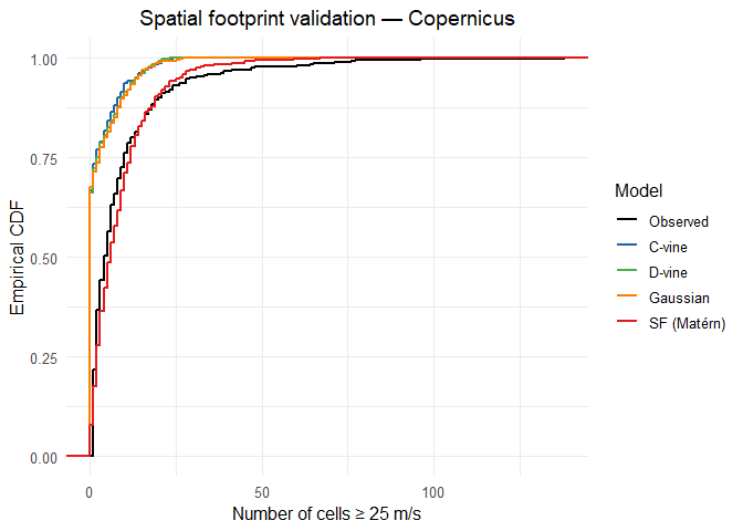

Empirical CDF of spatial footprint for observed data and four models.

How to read this plot. A model whose CDF curve lies close to the black “Observed” curve reproduces the spatial footprint well. A curve to the left means the model generates events that are too localised; a curve to the right means events that are too widespread. Use this plot to choose the model that best captures the dependence structure for your application.

Summary

Step	Goal	Key functions
Step 1	Read and standardize a gridded dataset	`hm_read_netcdf`, `hm_standardize_coords`, `hm_decode_time`
Step 2	Isolate extreme-event days	`hm_select_extreme_events`, `hm_to_matrix`, `hm_filter_land_cells`
Step 3	Fit a marginal distribution to each cell	`hm_fit_marginals`, `hm_pit_transform`
Step 4	Quantify spatial correlation vs distance	`hm_distance_matrix`, `hm_empirical_kendall`, `hm_empirical_correlogram`
Step 5	Fit copula or stochastic field model	`hm_fit_copula`, `hm_fit_correlation_model`
Step 6	Generate spatially coherent scenarios	`hm_simulate_copula`, `hm_simulate_sf_kle`
Step 7	Compare models against observed footprint	`hm_cluster_size`

References

Clavijo Mesa, M.V., Di Maio, F. & Zio, E. (2026a). A modeling framework for the inoperability assessment of interdependent critical infrastructures exposed to spatially distributed natural hazards. Reliability Engineering & System Safety, 275, 112830.

Clavijo Mesa, M.V., Broggi, M., Di Maio, F. & Zio, E. (2026b). Inoperability assessment of interdependent critical infrastructures exposed to natural hazards considering climate change. International Journal of Disaster Risk Reduction, 141, 106172.

Maria Valentina Clavijo Mesa

2026-10-06